Subsections

• Size$\to$ Half Size (Quick/simple) M
• Size$\to$ Half Size (Slower/accurate) M
• Size$\to$ Double Size M
• Size$\to$ Half Size X M
• Size$\to$ Half Size Y M
• Size$\to$ Arbitrary Resize... M
• Planar Transformations$\to$ Rotate $90^\circ$ [R] M
• Planar Transformations$\to$ Rotate $180^\circ$ M
• Planar Transformations$\to$ Rotate $270^\circ$ [Shift+R] M
• Planar Transformations$\to$ Rotate Arbitrary... M
• Planar Transformations$\to$ Flip Horizontal [H] M
• Planar Transformations$\to$ Flip Vertical [V] M
• Planar Transformations$\to$ Shift with Wrap... M
• Planar Transformations$\to$ Shear... M
• Planar Transformations$\to$ Rectify... M
• Spherical Transformations$\to$ Panoramic Transformations...
• Spherical Transformations$\to$ Diffuse/Specular Convolution... M
• Spherical Transformations$\to$ Ward Specular Convolution... M
• Spherical Transformations$\to$ Fast Diffuse Convolution (Lat-Long) M
• Spherical Transformations$\to$ Spherical Harmonic Reconstruct Lat-Long... M
• Spherical Transformations$\to$ Sample Light Probe Image to Light Source List... M
• Filter$\to$ Neighbor Average Blur M
• Filter$\to$ Gaussian Blur... M
• Filter$\to$ Bilateral Filter... M
• Filter$\to$ Motion Blur... M
• Filter$\to$ Horizontal Motion Blur... M
• Filter$\to$ Circle Blur... M
• Filter$\to$ Small Circle Blur... M
• Filter$\to$ Star Filter M
• Filter$\to$ Deinterlace M
• Filter$\to$ Incremental Adaptive Unsharp Sharpen [^] M
• Filter$\to$ Sharpen By... [Ctrl+6] M
• Filter$\to$ Laplacian of Gaussian... M
• Filter$\to$ X Derivative M
• Filter$\to$ Y Derivative M
• Filter$\to$ Gradient M
• Filter$\to$ Corner Detect M
• Filter$\to$ Edge Detectors$\to$ Gradient Based... M
• Filter$\to$ Edge Detectors$\to$ Laplacian of Gaussian Based... M
• Filter$\to$ Calculate Normals M
• Filter$\to$ Interpolate Bayer Pattern... M
• Filter$\to$ DCT (Discrete Cosine Transform) M
• Filter$\to$ IDCT (Inverse Discrete Cosine Transform) M
• Warp$\to$ Correct Lens Distortion M
• Effects$\to$ Vignette... M
• Effects$\to$ Randomize M
• Effects$\to$ Sepia tone... M
• Effects$\to$ Quantize M
• Effects$\to$ Signed Quantize M
• Effects$\to$ Vertical Cosine Falloff M
• Pixel$\to$ Set/Clear... M
• Pixel$\to$ Offset... M
• Pixel$\to$ Scale... M
• Pixel$\to$ Divide... M
• Pixel$\to$ Power... M
• Pixel$\to$ Exponentiate... M
• Pixel$\to$ Log... M
• Pixel$\to$ Replace Infinite/NAN... M
• Pixel$\to$ Round M
• Pixel$\to$ Floor M
• Pixel$\to$ Ceiling M
• Pixel$\to$ Desaturate M
• Pixel$\to$ Scale to Current Exposure [Ctrl+0] M
• Pixel$\to$ Clamp at Current Exposure M
• Pixel$\to$ Normalize M
• Pixel$\to$ Lower Threshold... M
• Pixel$\to$ Upper Threshold... M
• Pixel$\to$ Swap Byte Order [B] M
• Pixel$\to$ White-Balance Selection M
• Pixel$\to$ Scale Selection to White M
• Pixel$\to$ Compute Color Matrix...
• Pixel$\to$ Apply Color Matrix... M
• Pixel$\to$ Rasterize Triangle M
• Pixel$\to$ Index Map M
• Info$\to$ Max/Min/Average [I]
• Info$\to$ Copy Average [C]
• Info$\to$ Sample Grid...
• Crop M
• Calculate
• Duplicate [D]

`Image' menu

Size$\to$ Half Size (Quick/simple) M

Half-size an image by dividing the image into a square grid with each square containing 4 pixels. Simply take the average value of the 4 pixels and write out as one pixel. This method produces aliasing at boundaries of contrast in the image (cf. 10.2).

Size$\to$ Half Size (Slower/accurate) M

Half-size the image using a simple small blur kernel of size 1-2-1. This helps reduce aliasing which may be present if the Quick/Simple method is used(10.1). The image is blurred slightly in the horizontal direction for each consecutive 3 pixels with a 1-2-1 weighting function. This is repeated for the vertical direction, then a 'Half Size (Quick/simple) is done on the blurred image. The resulting image is thus slightly blurred such that simple half-size aliasing is diminished giving a less jagged result. The process is slightly slower due to the double blur operation.

Size$\to$ Double Size M

Double the width & height of the image. Uses bilinear interpolation of the existing values to infer the extra pixel values.

Size$\to$ Half Size X M

Reduce the width of the image by half from the average of consecutive pairs of pixels in each horizontal line in the image.

Size$\to$ Half Size Y M

Reduce the height of the image by half from the average of consecutive pairs of pixels in each vertical line in the image.

Size$\to$ Arbitrary Resize... M

Change the image dimensions to any values. Choosing this item prompts the user with a dialog allowing the dimensions to be specified along with choice of resizing method:

Changing the image width with the 'Keep Aspect Ratio' box checked causes the height to be automatically updated to maintain the same ratio of height/width as the original. Unchecking this box allows full control over the dimensions.

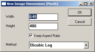
One of the following resizing methods is chosen (in order of increasing quality/decreasing speed):

1. Nearest neighbor interpolation:
   Pixel values from the old image are copied in to the nearest corresponding location in the new image regardless of the surrounding pixel values.
2. Bilinear interpolation:
   Uses the 4 surrounding pixels (horizontally and vertically) to interpolate values.
3. Bicubic interpolation:
   Uses the a weighted average $4\times4$ square of neighboring pixels from the original image to drive the interpolation. Weights are derived in terms of a cubic function.
4. BSpline interpolation:
   Uses the a weighted average $4\times4$ square of neighboring pixels from the original image to drive the interpolation. Weights are derived in terms of a BSpline function.
5. Bilinear Log interpolation:
   Uses the 4 surrounding pixels (horizontally and vertically) to interpolate values in Log space.
6. Bicubic Log interpolation [default]:
   Uses the a weighted average $4\times4$ square of neighboring pixels from the original image to drive the interpolation. Weights are derived in terms of a cubic function and in Log space.

Planar Transformations$\to$ Rotate $90^\circ$ [R] M

Rotate the image by $90^\circ$ clockwise.

Planar Transformations$\to$ Rotate $180^\circ$ M

Rotate the image by $180^\circ$ .

Planar Transformations$\to$ Rotate $270^\circ$ [Shift+R] M

Rotate the image by $270^\circ$ clockwise.

Planar Transformations$\to$ Rotate Arbitrary... M

Rotate the image by an arbitrary amount. The user specifies the amount of clockwise rotation in degrees. Note: the resulting image will be larger, reflecting the rectangular bounding rectangle that touches the rotated image corners. New pixels are set to black.

Planar Transformations$\to$ Flip Horizontal [H] M

Flip the image across the right vertical edge

Planar Transformations$\to$ Flip Vertical [V] M

Flip the image across the bottom horizontal edge

Planar Transformations$\to$ Shift with Wrap... M

Shift the image up or down and left or right. Pixels that are shifted off one edge are tacked on to the opposite edge ('wrapped').

Planar Transformations$\to$ Shear... M

Shear the image so that the bottom edge moves relative to the top. The amount of shear is selected as:

(bottom edge horizontal shift) $\div$ (image height)

The resulting image will be larger than the original to accomodate the bounding rectangle which touches the sheared image corners.

Planar Transformations$\to$ Rectify... M

Resample a quadrilateral area within the image to a rectangular image with the same or different dimensions. In order to rectify a quadrilateral area, first the area must be demarcated with 4 points (Shift+left-click) using the 'Point Editor' window (15.12). The 4 points must be arranged so that they form the quadrilateral when taken in anti-clockwise order beginning from the top-leftmost location. Select 'Image$\to$ Planar Transformations$\to$ Rectify' from the menu and give the desired output image dimensions. Rectification proceeds by computing the homography which maps the 4-point quad into the desired rectangular output. This homography maps all quad pixels into the output and then bilinear interpolation is used to fill in any gaps in the output.

Spherical Transformations$\to$ Panoramic Transformations...

Transform a panoramic source image into any of several useful other panoramic image spaces. See the online tutorials here for more information on these formats and an example of how to create a panormaic transformation.

The source/destination panoramic spaces can be any of:

1. Light Probe (Angular Map)
   
2. Mirrored Ball
   
3. Mirrored Ball Closeup
   
4. Diffuse Ball
   
5. Latitude/Longitude
   
6. Cubic environment (Vertical Cross)
   
7. Cubic environment (Horizontal Cross)
   

The 'Panoramic Transformations' dialog:

Procedure

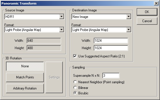
Choose the source image from the list of open images. Describe the panoramic format of the source image from the drop-down box as described above. Choose the target image or use the default behavior which is to create a new image. Choose the panoramic transformation format for the output image. Specify the output image dimensions, note the aspect ratio check box, and (optionally) specify a 3D rotation.

Spherical Transformations$\to$ Diffuse/Specular Convolution... M

HDR Shop can perform a diffuse or specular convolution on a high-dynamic range $360^\circ$ panoramic image (also called a light probe). This is useful if you need to pre-compute a diffuse or rough specular texture map; for example, to light an object using a light probe in real time applications. See the online tutorials here for more information. Note that the convolution is slow to process unless the input image is downsampled first.

Spherical Transformations$\to$ Ward Specular Convolution... M

Simulates a rough specular sphere lit by a light probe. The input and output images should be in lat-long format (see 10.16). Furthermore the input image must have width = 2$\times$ height and both width and height should be a power of 2 (eg 1024$\times$ 512). The output image will be a specular convolution of the input image or light probe using the specular BRDF Ward model. This is useful if you need to pre-compute a rough specular texture map; for example, to light an object using a light probe in real time applications. Lighting a specular surface with a preconvolved environment map produces a similar effect to lighting an actual rough specular surface with the original light probe. Note that the convolution is slow to process unless the input image is downsampled first.

Spherical Transformations$\to$ Fast Diffuse Convolution (Lat-Long) M

Simulates a diffuse sphere lit by a light probe. The input and output images should be in lat-long format (see 10.16). The output image will be a diffuse convolution of the input image or light probe using the Lambertian BRDF model. This is useful if you need to pre-compute a diffuse texture map; for example, to light an object using a light probe in real time applications. Lighting a diffuse surface with a preconvolved environment map produces a similar effect to lighting an actual diffuse surface with the original light probe. An example HDRShop script which performs the function can also be found here

Spherical Transformations$\to$ Spherical Harmonic Reconstruct Lat-Long... M

Approximates the input image/light probe as a sum of spherical harmonics up to the desired order. See this here for more information.

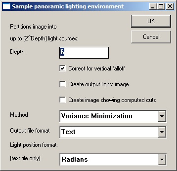
Spherical Transformations$\to$ Sample Light Probe Image to Light Source List... M

Samples a spherical lighting environment image into a number of areas where each area contains a single light source. Choice of areas and light source positions and intensities are computed based on the distribution of energy in parts of the image. In this way, the light source position and intensity most representative of each particular area is obtained. This is useful in rendering lighting environments where efficiency is paramount and a good approximation to the full resolution environment will suffice. The output is a text window listing the sampled positions and intensities in one of: plain text (spherical positions in radians or degrees, or as unit vectors on the sphere), Maya MEL script, or PBRT format, and also optionally either or both of: an image showing sampled pixel lighting locations and intensities; an image showing the subdivision areas of the image as a graph.

The 'Sample Panoramic Lighting Environment...' dialog:

See the online tutorials here for more information.

Filter$\to$ Neighbor Average Blur M

Each pixel is set to a weighted distance average of its immediate 8 neighbors. Performs very simple, very fast blur of fixed size.

Filter$\to$ Gaussian Blur... M

Apply a 2D Gaussian blur with specified kernel width in pixels

Filter$\to$ Bilateral Filter... M

Edge-preserving blurring filter. The filter weights the convolution in 2 domains so that the pixel is replaced with the weighted average of its neighbors in both space and intensity.

Filter$\to$ Motion Blur... M

Produces a linear blur with a selected width and at a selected angle chosen from a dialog box. Pixels are given the average value of all pixels (including subpixels) within the angled window with the given width.

Filter$\to$ Horizontal Motion Blur... M

Approximates horizontal motion blur by setting each pixel to be the average of pixels in a window with width specified in the dialog box. Optimized to be faster than motion blur with arbitrary direction.

Filter$\to$ Circle Blur... M

A simple blur filter which creates a circular kernel with the radius given in the dialog box. The values within the kernel sum to 1. The image is then convolved with this kernel. The kernel format is such that inside the circle, the values are the same everywhere and the edge pixels fall off smoothly from this value (akin to a Gaussian blur with minimal spread).

Filter$\to$ Small Circle Blur... M

A simple blur filter which creates the following $5\times5$ circular kernel:

$\left[ \begin{array}{ccccc} 0.000000 & 0.015873 & 0.039683 & 0.015873 & 0.0000... ...73 \\ 0.000000 & 0.015873 & 0.039683 & 0.015873 & 0.000000 \end{array} \right]$

to produce a weighted circular distance average value for each pixel.

Filter$\to$ Star Filter M

Generates s vertical and horizontal star-shaped blur approximating simple image glare.

Filter$\to$ Deinterlace M

Removes common 'tearing' artifacts in deinterlaced images by doing a simple 1-2-1 weighted vertical blur on the consecutive interlaced fields.

Filter$\to$ Incremental Adaptive Unsharp Sharpen [^] M

Do a small incremental sharpen on the image using the 'adaptive unsharp sharpen' method:

New image = Original image + Convolve(original image, kernel) where kernel =

$\frac{1}{16}\times\left[ \begin{array}{ccc} -1 & -2 & -1 \\ -2 & 12 & -2 \\ -1 & -2 & -1 \end{array} \right]$

Filter$\to$ Sharpen By... [Ctrl+6] M

Sharpen an image by a specified amount using one of 5 convolution kernels.

Choose an amount to sharpen by, a method, and whether to clamp the sharpened values to within the same range as the input image. The methods specify different convolution kernels to use in the sharpening process. Note that the default settings do the same as the 'Incremental Adaptive Unsharp Sharpen' (10.31) filter.

Filter$\to$ Laplacian of Gaussian... M

Alternative sharpening filter. The Gaussian operation smoothes noise. The Laplacian part enhances edges by both down-weighting and up-weighting the opposing values across an edge. The image is filtered by a LoG filter and the result is added to the original image to produce the sharpening.

Filter$\to$ X Derivative M

Computes the local gradient in the X direction based on the x-1,x+1 values.

Filter$\to$ Y Derivative M

Computes the local gradient in the Y direction based on the y-1,y+1 values.

Filter$\to$ Gradient M

Filter the image according to $\sqrt{dX^2 + dY^2}$ where dX is the X-derivative filter 10.34, dY is the Y-derivative filter 10.35

Filter$\to$ Corner Detect M

A simple corner detection filter which convolves the image with the $5\times5$ kernel:

$\left[ \begin{array}{ccccc} -1 & -1 & 0 & 1 & 1 \\ -1 & -1 & 0 & 1 & 1 \\ 0 ... ...& 0 & 0 & 0 \\ 1 & 1 & 0 & -1 & -1 \\ 1 & 1 & 0 & -1 & -1 \end{array} \right]$

Filter$\to$ Edge Detectors$\to$ Gradient Based... M

A simple edge detector which produces a binary image depicting edges according to the chosen threshold value. The filter simply does a 'Gradient' filter (10.36) operation and then sets pixels above the threshold value to white, otherwise to black.

Filter$\to$ Edge Detectors$\to$ Laplacian of Gaussian Based... M

Alternative edge detector based on 'Laplacian of Gaussian' filter (10.33). The LoG filter produces an image where values across an edge are positive on one side and negative on the other. The filter then simply computes the zero-crossing points and sets those with sufficiently high gradient to white, otherwise to black.

Filter$\to$ Calculate Normals M

Computes a field of surface normals from the input image assuming that the input image represents a point cloud of values in x,y,z so that x = r, y = g, z = b. The normals are then computed based on the neighboring 'x,y,z' values.

Filter$\to$ Interpolate Bayer Pattern... M

Interpolate RAW digital camera single channel image into 3 channel image.

Most common high-end digital camera sensors record an image under a color filter array of red, green and blue filters in one of 4 possible arrangements called a Bayer pattern. The filter pattern is a mosaic of 50% green, 25% blue and 25% red. Uninterpolated RAW images are thus single channel, but can be interpolated to 3 channels using the known Bayer pattern.

Possible Bayer patterns:

• RGGB
• BGGR
• GRBG
• GBRG
  
  

Two interpolation algorithms are available in HDR Shop:

• Adaptive Homogeneity Directed (AHD):
  A relatively new technique which constructs a homogeneity map of the image and uses that map to choose which direction to interpolate in. This significantly reduces color artifacts compared to other techniques.
• Second-Order Gradient:
  Evaluates gradients around the pixel of interest and makes a smoothness estimate based on the lower of these gradients. Suffers from color artifacts. Recommended to use AHD above
  
  

Filter$\to$ DCT (Discrete Cosine Transform) M

Convert an image from the spatial domain into the frequency domain

Filter$\to$ IDCT (Inverse Discrete Cosine Transform) M

Convert an image from the frequency domain into the spatial domain

Warp$\to$ Correct Lens Distortion M

'Undistort' the image using the given optical calibration parameters.

Correct Lens Distortion dialog:

The user either specifies the calibration parameters manually or loads them in via a 'Matlab' (*.m) file with the correct internal format.

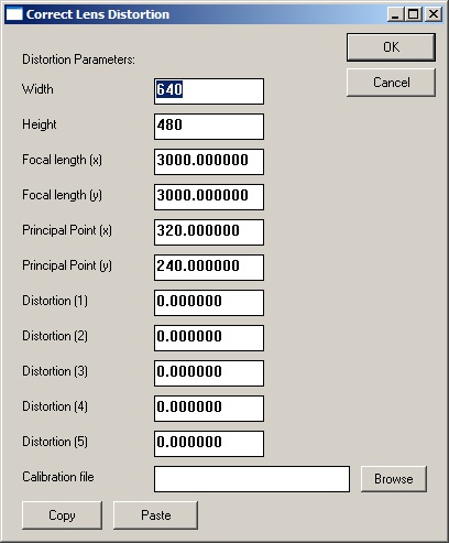
Description of distortion parameters:

• Width: input image width
• Height: input image height
• Focal length (x): focal length of the lens in pixels
• Focal length (y): focal length of the lens in pixels
• Principal Point (x): point through which the Center of Projection passes (usually the center of the image)
• Principal Point (y): point through which the Center of Projection passes (usually the center of the image)
• Distortion (1): Radial distortion
• Distortion (2): Radial distortion
• Distortion (3): Radial distortion
• Distortion (4): Tangential distortion
• Distortion (5): Tangential distortion
  
  

Alternatively, a Matlab or text file (*.m) may be read in to set these parameters so long as the file contains the requisite information according to the following schema (order of lines in the file does not matter):


kc = [ $<r_1>$ ; $<r_2>$ ; $<r_3>$ ; $<t_1>$ ; $<t_2>$ ];
fc = [ $<f_x>$ ; $<f_y>$ ];
cc = [ $<c_x>$ ; $<c_y>$ ];
nx = $<width>$ ;
ny = $<height>$ ;


Where:

• $r_n$ = radial distortion parameters
  
• $t_n$ = tangential distortion parameters
  
• $f_x/y$ = focal length x/y
  
• $c_x/y$ = principal point x/y
  
  

Click 'OK' and the parameters are used to undistort the image.

Effects$\to$ Vignette... M

Darkens image close to the edges based on the radius value entered in the dialog box. Used for generating an 'old-fashioned movie camera' appearance.

Effects$\to$ Randomize M

Set the image pixel channels to have random values between 0 and 1.

Effects$\to$ Sepia tone... M

Apply a color tone to a black-and-white version of the image. A color-picker dialog is displayed and the user chooses the tone. The single channel intensity 10.62 version of the image is then computed and the pixels values are multiplied by the chosen tone.

Effects$\to$ Quantize M

Rescale the image into the specified number of discrete values.

Effects$\to$ Signed Quantize M

Rescale the image into the specified number of discrete values allowing for negative values.

Effects$\to$ Vertical Cosine Falloff M

Applies a cosine scale to each pixel based on the pixel's vertical location. This is used to scale an image into an equal-area weighted representation. eg lat-long images generated in HDRShop like some World Map projections, are stretched at the poles (top & bottom) so that those pixels are over-represented relative to those at the equator (mid-horizontal line of pixels).

Pixel$\to$ Set/Clear... M

Set the pixel channel values within the selected region to the values specified in the dialog.

Pixel$\to$ Offset... M

Increment/decrement the pixel channel values within the selected region by the values specified in the dialog.

Pixel$\to$ Scale... M

Multiply the pixel channel values within the selected region by the values specified in the dialog.

Pixel$\to$ Divide... M

Divide the pixel channel values within the selected region by the values specified in the dialog.

Pixel$\to$ Power... M

Raise to a power the pixel channel values within the selected region by the values specified in the dialog.

Pixel$\to$ Exponentiate... M

Raise the values specified in the dialog to the power of the pixel channel values within the selected region.

Pixel$\to$ Log... M

Take the Logarithm of the pixel channel values within the selected region in the base of the values specified in the dialog.

Pixel$\to$ Replace Infinite/NAN... M

Replace any non-real values with a real value within the selected region.

Pixel$\to$ Round M

Replace values greater than or equal to 0.5 with 1, and values less than 0.5 with 0 within the selected region.

Pixel$\to$ Floor M

Round the channel values down to the next lower integer value within the selected region. eg $0.99 \Rightarrow 0$ and $-2.3 \Rightarrow -3$

Pixel$\to$ Ceiling M

Round the channel values up to the next higher integer value within the selected region. eg $0.2 \Rightarrow 1$ and $-2.3 \Rightarrow -2$

Pixel$\to$ Desaturate M

Desaturate the selected pixel values according to the weighting scheme in http://www.sgi.com/misc/grafica/matrix/.

The weights used are:

D = 0.3086 $\times$ red + 0.6094 $\times$ green + 0.0820 $\times$ blue

Note that these values are distinct from computing 'Intensity' used elsewhere in the software, which we take as being:

I = 0.299 $\times$ red + 0.587 $\times$ green + 0.114 $\times$ blue

Pixel$\to$ Scale to Current Exposure [Ctrl+0] M

Set the channel values to the exposure in the current display within the selected region. Every +1 stop will double the channel value.

Pixel$\to$ Clamp at Current Exposure M

Set the channel values to the exposure in the current display within the selected region. Every +1 stop will double the channel value. Set new channel values of greater than 1 to 1 and divide all channel values by $1 \div (exposure multiplier)$ . eg a value of 0.5 clamped at a current exposure of +3 stops will get set to $0.5 \times 2^3 = 4$ initially, then clamped to 1, then divided by $2^3$ to finally give 0.125.
Used to show the effect of losing some of the dynamic range in an HDRShop image.

Pixel$\to$ Normalize M

Normalize per pixel channels. eg red channel = $\frac{(red channel)}{\sqrt{(red channel)^2 + (green channel)^2 + (blue channel)^2}}$

Pixel$\to$ Lower Threshold... M

Set pixel values of less than the chosen thresholds (per channel) to the threshold values within the selected region.

Pixel$\to$ Upper Threshold... M

Set pixel values of greater than the chosen thresholds (per channel) to the threshold values within the selected region.

Pixel$\to$ Swap Byte Order [B] M

Swap the byte order in the case that the current image was created on a system with a different byte order regime.

Pixel$\to$ White-Balance Selection M

Leverage an area known to be white or gray in the image to color balance the rest of the image. This is useful where one or more of the channels in the image are overly high.
Procedure: Select an area known or assumed to be any shade of gray up to white and select this menu item. HDR Shop computes the mean channel values within the selected region, takes the intensity (10.62) of the mean values and divides the intensity by the mean channel value, then multiplies each channel in the whole image by the result of that division for that channel. When this is applied, the average channel values in the selected region will now be almost identical (ie gray-white) and this correctional scaling will have been propagated to the rest of the image.

Pixel$\to$ Scale Selection to White M

Leverage an area known to be white in the image to color balance the rest of the image. This is useful where one or more of the channels in the image are overly high.
Procedure: Select an area known or assumed to be white and select this menu item. HDR Shop computes the mean channel values within the selected region then each channel in the whole image is scaled by the reciprocal corresponding mean channel value. When this is applied, the average channel values in the selected region will be almost exactly 1 and this correctional scaling will have been propagated to the rest of the image.

Pixel$\to$ Compute Color Matrix...

Compute the $3 \times 3$ matrix which maps channel values in one image to those in another image. This function can be used for recovering the overall color change between 2 versions of the same image after one version has been altered by some unknown sequence of transformations. It is more commonly used in conjunction with a Macbeth Color Chart to color balance images or to transform images into a particular color space (eg sRGB or AdobeRGB).

Procedure:

Requires 2 images of the same size to operate on. Select the source and target images from the dialog and click OK. HDR Shop solves by creating a system of linear equations from each pixel channel. This system is then solved by finding the pseudo-inverse using SVD. the resulting $3 \times 3$ matrix is presented as a dialog. From here the matrix or constituent parts can be copied to the text buffer.

See this tutorial for more information.

Pixel$\to$ Apply Color Matrix... M

Change the pixel values in the image via a $3 \times 3$ matrix. Any custom matrix, row or column can be pasted in to the dialog before applying it to the channel values.

See this tutorial for more information.

Pixel$\to$ Rasterize Triangle M

the user specifies a triangle in three points using the point editor (15.12). Triangle is textured using barycentric coordinates with R, G, B at vertices.

Pixel$\to$ Index Map M

Stores the image pixel coordinates in the red and green channels.

Info$\to$ Max/Min/Average [I]

Show Maximum/Minimum/Average/Sum/RMS error information about the selected area. Note: if no area is selected, information for the whole image is shown. Average channel values are the mean. Pixel channel values can be copied to the text buffer. Pixel locations for maximum and minimum channels are shown beneath the values.

Info$\to$ Copy Average [C]

Copy the mean channel values within the selected region to the text buffer.

Info$\to$ Sample Grid...

This function is used to create a grid sampling of colors which represent the mean values within the image or selected area. Typically this is used to color balance an image against a reference set of known colors such as a Gretag-Macbeth color chart.

Procedure:

There are 2 available methods for obtaining the sample area:

Pre-rectify method:
If the image of the color chart was not orthogonal to the camera you can rectify the chart as a rectangle by first selecting the 4 grid corner points. Mark the 4 corners (Shift+left-click) in a counter-clockwise pattern starting with the top-left corner.
Drag-select method:
Select the area of the image to be sampled or just leave blank if using the whole image.

Select the Image$\to$ Info$\to$ Sample Grid... dialog. Enter the grid dimensions and the number of samples (horizontally & vertically) to be taken from the center of each grid square. 10 samples in width and height will cause the $10 \times 10$ square in the grid square center to be used as the samples. If you are rectifying the image first, a 'Use points to rectify rectangle first' checkbox will be shown and checked automatically. On clicking 'OK', an intermediate rectangular image is computed from the homography between the corresponding sets of corners and this image is then used as the input to the sampling algorithm. The mean value for each set of grid square samples is computed and output as an image with one pixel for each grid square with the value of the mean of the samples within the input grid.

See this tutorial for more information.

Crop M

Crop the image to the selected area. Either select an area with a 'left-click and drag' operation or with the 'Select$\to$ Show Selection Area Window' ('S' key 13.3). Select 'Crop' from the menu to complete the operation.

Calculate

Perform various math operations on between one & four of the currently open images.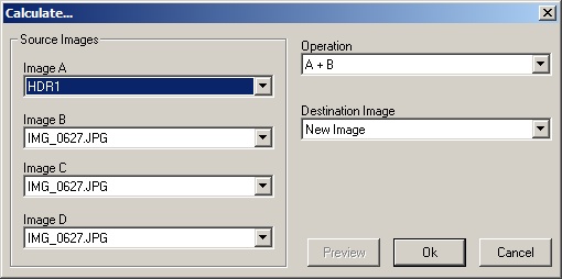

Available operations (images used in operation):

• Addition (A,B) Add A and B
• Subtraction (A,B) Subtract B from A
• Multiplication (A,B) Multiply A and B
• Division (A,B) Divide B by A
• Absolute Magnitude (A) Absolute pixel values in A
• $A \times C + B \times (1 - C)$ (A,B,C) Blend A and B weighted by C (alpha blend of B & A with C as the mask)
• Addition (A,B,C,D) Add A, B, C and D
• Panorama Blend (A,B,C,D) Compute the mean pixel value across all 4 images.
• Maximum (A,B,C,D) Find the maximum values at each pixel in all four images
• Minimum (A,B,C,D) Find the minimum values at each pixel in all four images
• 1 minus image (A) Compute (1 - A)

The output image name reflects the operation that was performed for clarity.

Duplicate [D]

See 'Window$\to$ Duplicate' (15.1)